Verifying calibration result – is it any good?

So, you have generated a calibration params file, and wonder how to determine if the quality is good?

Well, the first thing to do, is to connect the board to a ground control station (PC or Android) and open up the HUD. In most cases, the artificial horizon will be off for a new board. In the odd case that you have a level horizon, you should still calibrate in order to secure that the board is fully compensated for temperature changes and scales are correctly calibrated. What works on your desk inside your house at 20C, may be way off at another temperature.

Now, load your calibration parameters and click “save to ROM”. As you do this, you should see the artificial horizon begin to line up, but it may not be spot-on, before the board has been reset or power-cycled. After a reset, the horizon should be level when the board is level and respond accurately to movements of the board.

If the horizon does not line up after a reset, that is the first indication that your calibration parameters are wrong.

If you want to dive more into the individual sensors, you can do this by comparing the sensor’s before and after values by making some log files to compare the uncalibrated and calibrated state of the board.

Part 1: Verify Magnitudes and Magnetometer influence

A quick “sanity check” of the calibration is to verify the “magnitude” values for the Accelerometer (ACC) and Magnetometer (MAG) sensors.  This can tell you how close to “level” the AQ thinks it is while in different orientations.  To do this, use the Diagnostic Telemetry view in QGroundControl-AQ.  Go to the Values Chart, connect to your AQ, and hit Start Telemetry button (update freq. 100 is good, a wired connection is recommended).  Set the Time Span to something like 20s or 30s.

Now, first check the ACCs. Select ACC Magnitude checkbox in the list on the left.  Place your AQ level and note the magnitude value in the graph.  It should be very close to 9.8 (1 Earth gravity), with very little variance (short “jaggies”).  Now turn the AQ on one side and keep it steady (or, better, set it down… in fact it doesn’t have to be perfectly at 90 degrees, anywhere close is fine).  The magnitude should vary while you are moving the AQ, but quickly settle back to 9.8 once movement stops.  Try the same with the rest of the sides (and upside down).  If you find that it doesn’t consistently return to 9.8, that means the calibration is not perfect.  If the ACC magnitude varies within 9.7 to 9.9 or so, you’re fine. 9.6 to 10 is OK, not great.  It might be impossible to get it perfect, so don’t spend too much time on that.

Here’s an example… flat, 3 sides, then upside down (all hand-held, so a bit rough too). OK, but not great (click for full size):

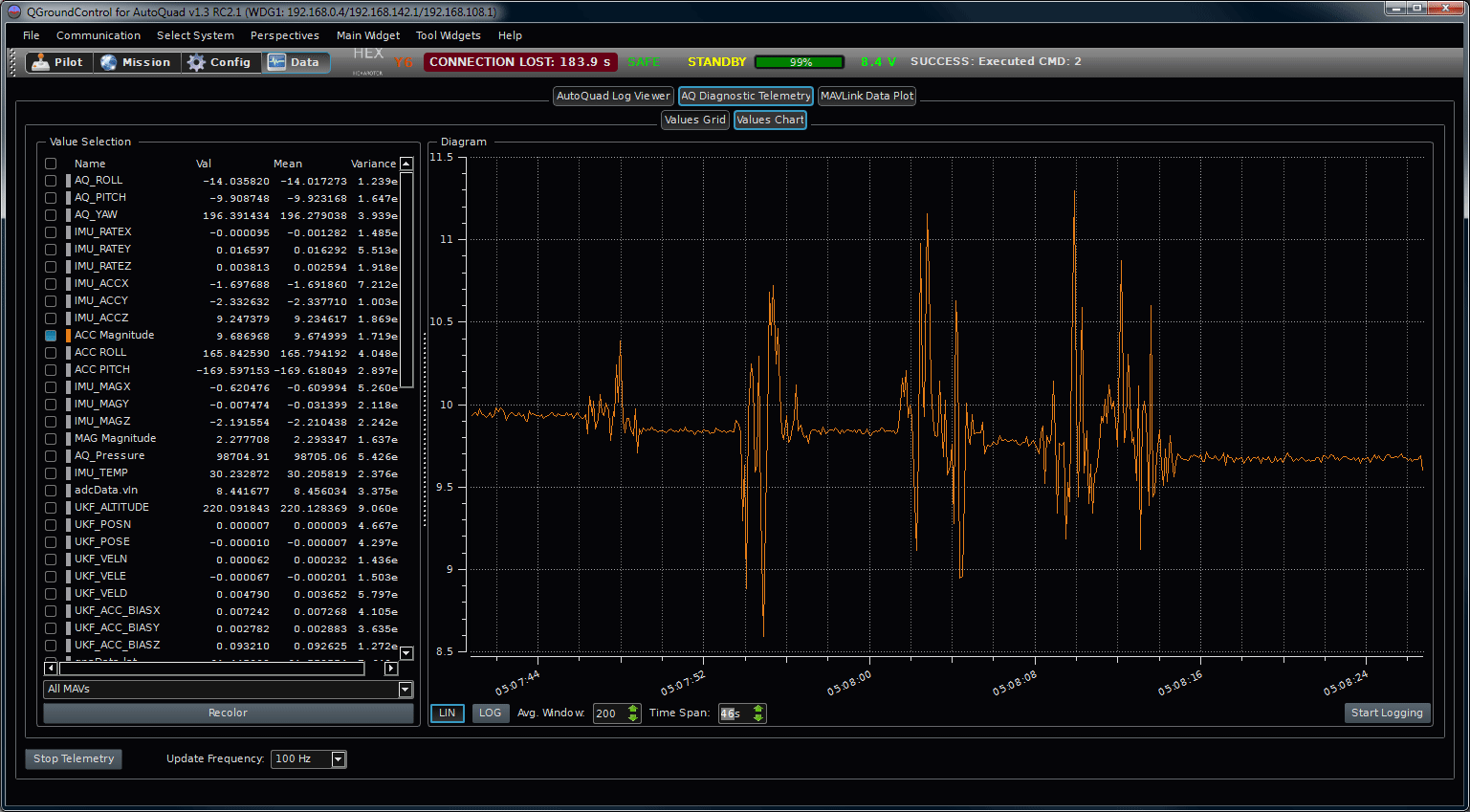
Now you can do the same with MAG Magnitude.  The value you’re looking for here is 2 (the representation of Earth’s magnetic field).  Again don’t worry if it’s not perfect, but between 1.95 and 2.05 is nice.

Note that while you’re actually flying, the AQ probably won’t get anywhere near 90 degree tilt, and certainly not upside down (if it does, you have bigger issues! 🙂 ).  The most important values are the ones around flat (right side up), and +/- 45 degree tilt in each direction.  Also what is most important is the change between the magnitudes at different orientations, not so much the actual value (though closer to 9.8 or 2.0 is better).  The magnitude values should be close to 9.8/2.0 when the AQ is held steady in any orientation.

As a final check, with the board mounted in your frame, you can compare AQ_ROLL and AQ_PITCH with ACC ROLL and ACC PITCH.  The former are what the AQ has derived based on ACC and MAG sensors.  The latter are derived purely from ACCs.  This can tell you how much of an effect the MAGs are having on the final solution.  This is more useful to determine if your frame/construction might be having a negative effect on the MAGs.  If you’re daring and careful, you could try this with motors running (to test the effect of your power distribution system under load).

Part 2: Temperature compensation

The first part is to check the temperature compensation of the 3 sensors. The basic procedure is to collect a static log and check that the sensor values do not drift as the board heats up.

To do this, put your board back into your logging container and collect a static log for 15-20 minutes or longer. A purist will of course repeat the whole freezing procedure and verify the whole temp range compensation, but if you catch a range of 15-40C that will still give a good representation by which to judge the temp compensation.

Now load the 15-20 minute static log file and graph the 3 IMU_RATE values.

You should see that they stay close to 0 as the board heats up. The filters will be able to handle some deviation, but if you see massive spikes or shifting zero-point of the rates, then there is a problem somewhere in the calibration. It should look something like this with nice flat curves:

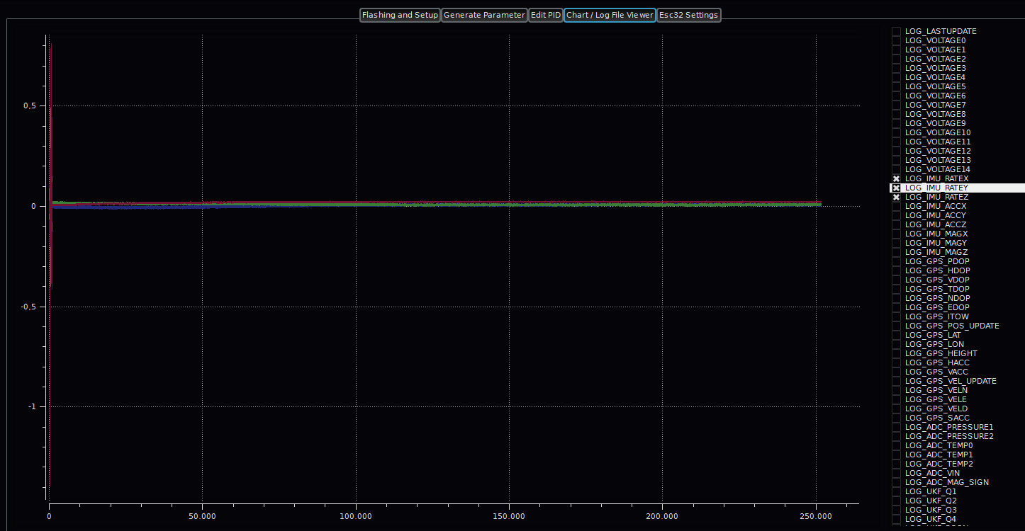
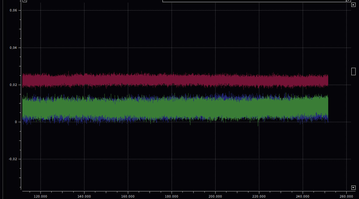
If you zoom in you should see deviations less than 0.05 for each axis:

Same procedure for the IMU_ACC values:

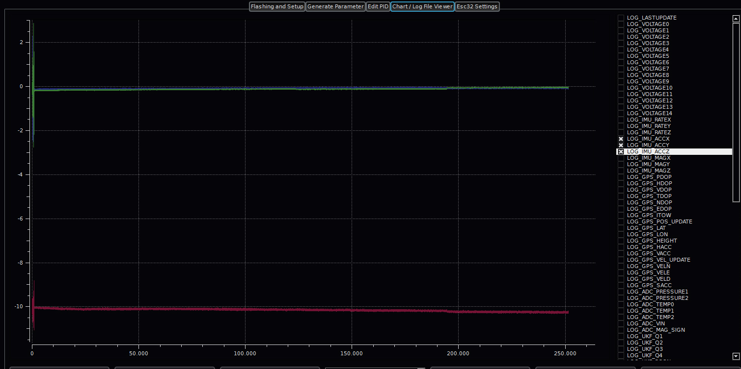
Actually the above example is NOT ideal, as we can see the Z-axis drifts  ~ -0.2 over this temperature, meaning an error of about 0.2m/s^2 is being added over this range. This board should probably be re-calibrated. You should aim for less than +/- 0.1 deviation on each axis. This is from a flying solution, but its not ideal!

We do the same thing again for the magnetometers:

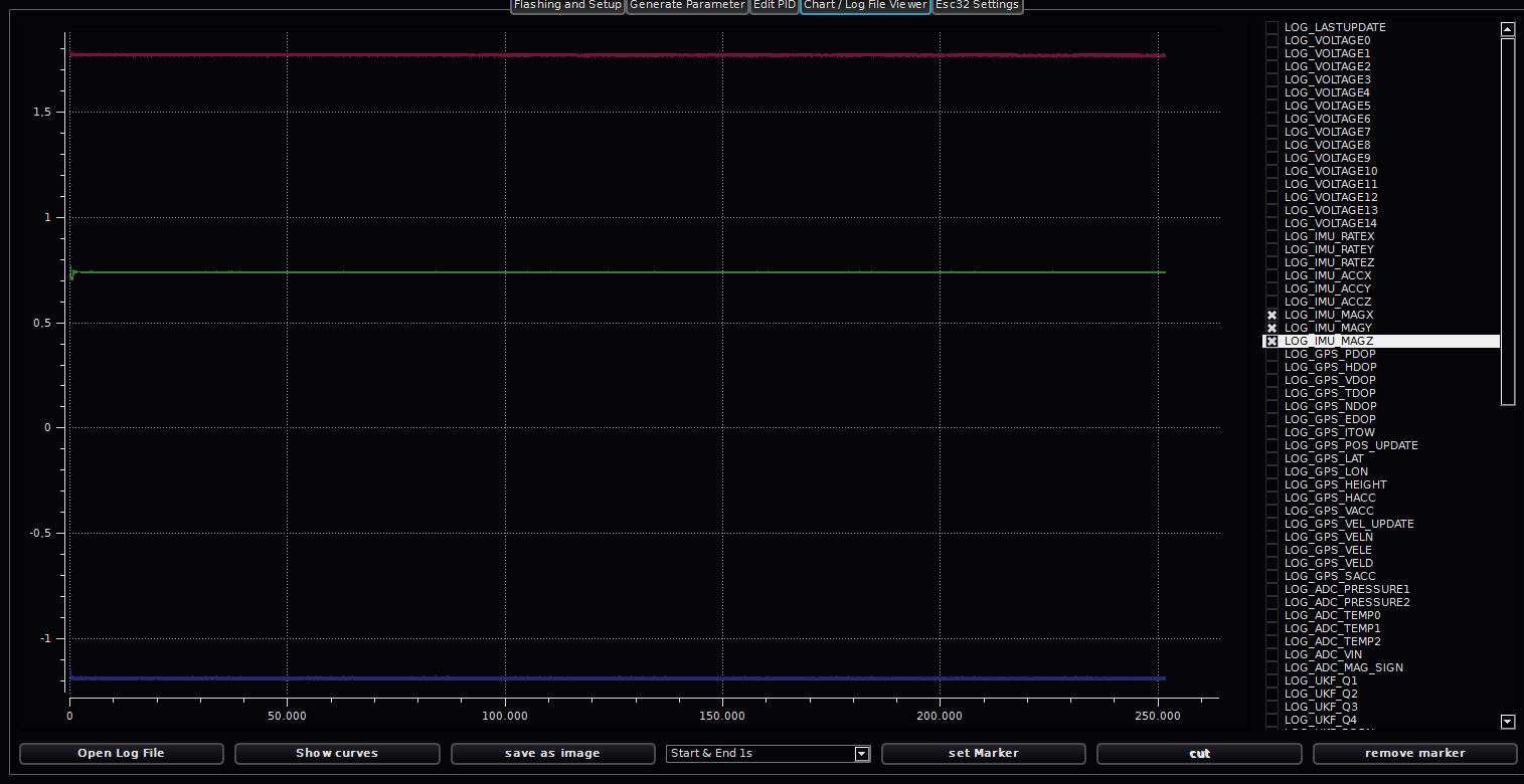
The above example is very close to ideal. We see nice flat curves and very little deviation of less than 0.05, meaning that the magnetometers was compensated very well.

Part 3: Scale and Bias

It is important to remark that the calibration procedure is an approximation, and without access to very expensive rate tables and magnetic “silent” environments we can not make a 100 percent accurate bias and scale measurement of each axis.

But we can do some short logs and use those to get an idea of the scales and bias. To prepare for this, mount the board on standoffs that will allow you to place the board level and upside down:

Then create some logs ~1 minute long of the board in uncalibrated and calibrated states (note: you could also use the live Telemetry graph view described in Part 1 while logging, though having wires attached could make this more difficult):

1. Insert a uSD card and boot up the board in level position. Keep it level for 15-20 seconds and make sure its not disturbed.
2. Then turn the board upside down and let it log for another 15-20 seconds.
3. Finally, turn the board slowly 360 degrees on all 3 axises. Return to level and disconnect power.

Load your calibration parameters to the board, and repeat this procedure. That will give you two logs — before and after calibration.

Checking the Gyros

Gyros can not easily be estimated if we don’t know EXACTLY how fast the board is turning. This is not possible to know without access to lab-quality rate tables.

In case of the gyros, there wont be any visible difference in the two log files – you might see some scale difference, but that might as well be because you turned the board at different speeds.

You should just confirm that all 3 axises are 0 and that they move away from 0 when the board is turned.

Checking the accelerometers

The accels are a very important component in the estimation of acceleration and speed of the craft, and it is essential to have a very well calibrated accelerometer if you want to achieve pinpoint accuracy and navigation speeds. Luckily the accels are easy to check by measuring the range and zero-point of each axis with the board at different orientation to the Earth’s gravity field (1G). In this example we just verify the Z axis range, by looking at the two 1-minute files we created earlier.

But If you make a jig or frame that will allow to set the board at exact 90 degree angles to the earth you can apply the same principle to the X and Y axises and verify that Z is 0 when the board is at 90 degrees to the ground.

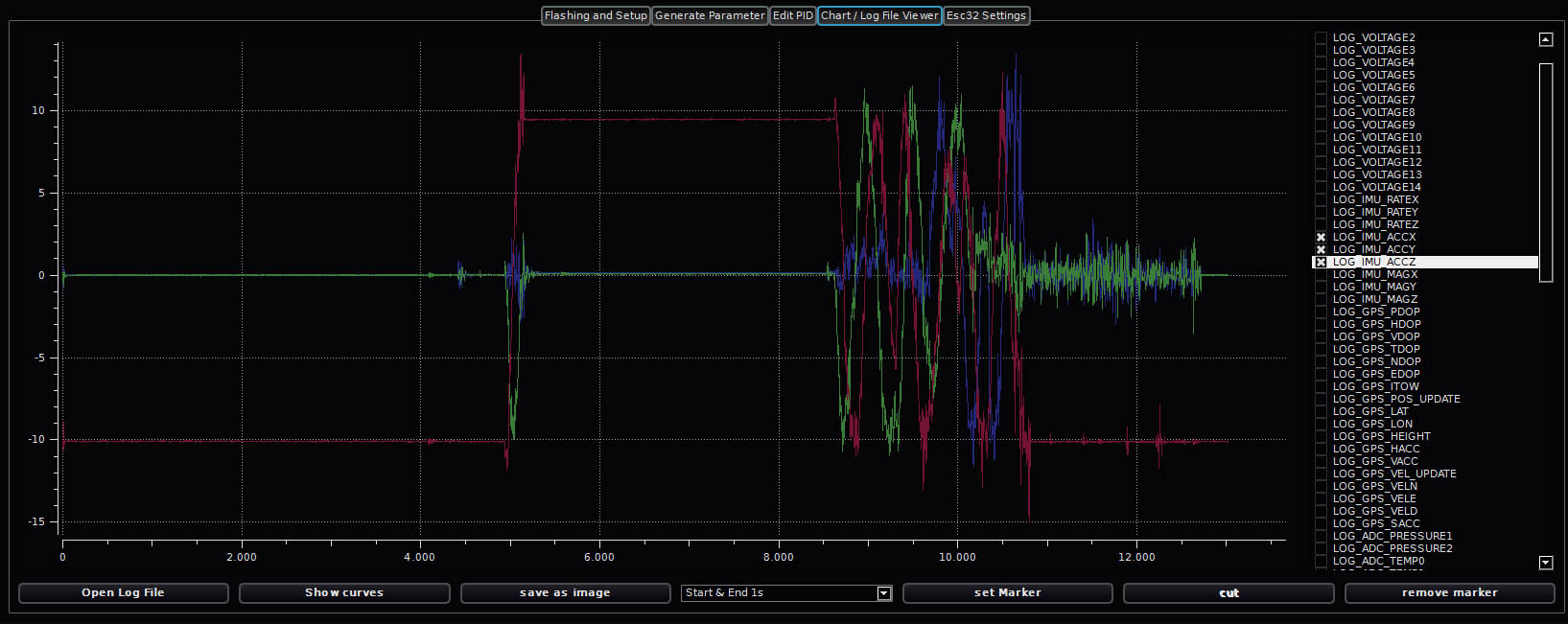
Load the uncalibrated log file into the log viewer and plot the 3 accel axes:

With the board level, we see that X and Y (Green and Blue) are not 0 and that Z (red) is around -8.5 at level and roughly 11.5 when upside down. We are looking for 0 on X and Y and as close to +/- 9.806 (1G) on the Z axis as possible. This uncalibrated result will produce an offset in the level estimations and probably also in the vertical and horizontal speed measurements — not good.

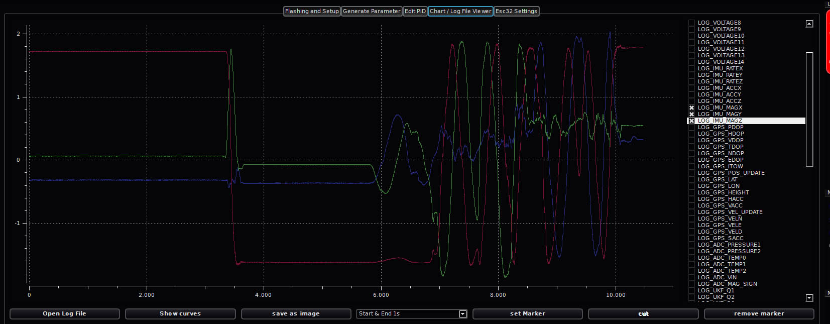
Here is the same board after calibration:

Notice that X and Y are very close to 0 and that Z is now showing a scale from around -10.1 to 9.5 (total range is 19.6). Remember that we were expecting to see 1G as 9.806, so the total range of 19.6 equates pretty well. However there is still an offset (bias) of about 0.3. The absolute ideal is to see a range of -9.806 to 9.806 with a tolerance less than 0.005. But that is very hard to achieve with the manual techniques available to us. Ideally, you should aim for deviations of less than 0.1. Note that you need an absolutely level surface to place the board on to make this test and the table used for this session was a bit off level. Check with a spirit level.

This is a good example of how a seemingly small bias can lead to a lot of error. With an error of 0.3 m/s^2 , for every second that passes, your velocity will be off by an additional 0.3 m/s. Left uncorrected, after 10 seconds the accel velocity would erroneously report 3 m/s while continuing to grow. The altitude estimate will get much worse than that, much faster.

Trivia: If the board is left sitting un-powered in the same position for prolonged time, the proof mass of the accel sensors tends to droop over time as gravity pulls on it. What was calibrated perfectly well, might be off by quite a bit a few months later if the board has been sitting in the same orientation. Any sort of hard impact or crash can bend things as well – enough to want to do another calibration. So exercise your craft regularly and remember to check the accels if you left it hanging in the same place for prolonged periods without flying (several months).

The key to getting “near-perfect” results for the accel calibrations is good log files, especially the dynamic dance is important to get right. But you should also check the static files and make sure you don’t have any spikes or noise in the voltage plots for the accels.

Estimating the Magnetometers

This is where is gets tricky. Magnetometers are subject to interference from metallic objects and electrical current paths in the near vicinity — the bigger the object or current is, the further you need to remove yourself from it!

So unless you have access to a lab environment with no significant magnetic interference and a nonmagnetic rate table, the best thing you can do is to go outside, away from large metallic objects or electronic circuits and make some measurements there. Remember to remove belt buckles and other metallic or electronic objects from yourself as well. Ideally you should perform the magnetometer test with the board mounted in the powered frame and in the same place where you did the Calibso calibration dance.

An ideally calibrated magnetometer will show a range of +/- 2.0 when turned 360 on all 3 axises. However, as the sensors is subject to interferences from a lot of sources, you can expect to see the ranges and scales change with location – ranges of up to +/- 2.7 have been observed when working the boards near sources of interference. The filters are able to handle some offset and scale change, so just verify that you are getting roughly the same range and scale for each magnetometer axis as you turn the board.

Here is an example of a calibrated board:

We can verify that the ranges are close to +/- 2.0 and that they roughly have the same range on each side of zero – deviations can be as high as 20 percent over the whole range. Again, this is hard to measure 100 percent precisely, so use your common sense to judge the solution! If you see any scale being way off, it could point to problems with your calibration but it could also just be a source of interference that is messing with you so before you throw out your params and begin again, try and relocate and make another log.

If your compass indicator is showing correct heading in flight, you probably got it right!

Getting it right matters

The Unscented Kalman Filter (UKF) used in AutoQuad, is capable of handling a lot of error in the sensors and relies on the GPS and barometer to correct. We have seen examples of completely uncalibrated board that flew seemingly well as long as there was good GPS reception. But you should not underestimate the need for calibration and you should always test that your craft flies well without GPS reception (disconnect antenna). The UKF will do an excellent job of hiding problems up to a certain point where the errors become critical and bad things begin to happen.

Basically the job of the UKF is to figure out that there is a bias and estimate it on each of the 3 ACC axes as well as 3 GYO axes. If this cannot happen quickly enough before you try to engage altitude hold, your craft will drop as the FC thinks it is rising. With the absolute information from the GPS and pressure sensor readings it is usually able to do the job well. The problem with all of this is that the UKF now knows that there is a lot of variance in the ACC biases so it effectively learns to trust these sensor readings less. This hurts its ability to adapt to, and properly estimate other states. In the end, there is no substitute for very well calibrated sensors no matter how good of a state filter you have.